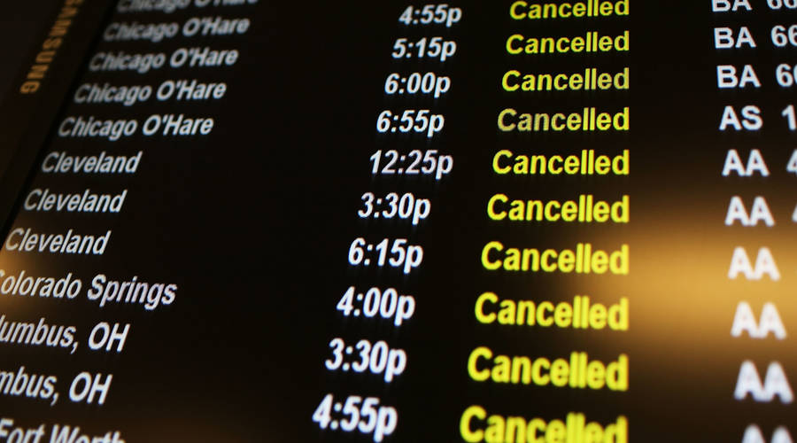
Over 99% of all scheduled domestic flights take off, and the rest are very expensive. Of over 10 million scheduled flights each year, hundreds of thousands never leave the tarmac. At an average of $5,770 in losses per cancellation this adds up to nearly a billion dollars of opportunity. While a significant chunk of those losses is unavoidable, it stands to reason that if an airline could confidently predict a cancellation far enough in advance, they could start taking measures to reduce those losses by doing such things as rebooking stranded passengers and rescheduling flight crews.

Abstract

The aim of this project is to build a model capable of predicting flight cancellations at least 24 hours in advance of the scheduled departure time. The premise behind this is that within sufficient foresight of an impending cancellation, an airline can take preemptive measures to reduce the ensuing cost and misery for all involved. To do this, I constructed a dataset of over 12 years of flight records and weather data for the same period and trained machine learning algorithms to predict future flight cancellations based on these historical observations. While this article will give a broad overview of the project and touch on some of the more interesting problems within, you can also see a full walkthrough of the code and model development in this notebook on my Github.

Data Sources

Flight Records

My data set is primarily derived from the "Marketing Carrier On-Time Performance" database hosted by the Bureau of Transportation Statistics, which contains information on nearly every flight conducted by a significant U.S. carrier dating back to January 1987. As that amount of data is pretty unwieldy for a prototype, for the purposes of this project I've narrowed the scope to only making predictions on flights departing from my home airport, the Seattle-Tacoma International Airport, from 2007 to the end of 2018.

Weather Records

To supplement the flight data, the model also makes use of historical weather data for the same time duration. This weather data is acquired via the Dark Sky API, and gives hourly records of precipitation, temperature, wind, visibility, and more. I couldn't, unfortunately, find a resource for historical weather forecasts, so I ended up using a combination of day-before weather observations and constructing a proxy for forecasts by adding noise to actual observations from the day of flights.

Future Data Sources

There are a number of additional features that this model would likely benefit from that have not yet been incorporated. Likely future resources include aircraft specific features that can be acquired by cross referencing with this database from the FAA.

Tools

Data Management

• Postgresql
• Sqlalchemy
• Psycopg2

Code

• Python
• Jupyter notebook

Data exploration and cleaning

• Numpy
• Pandas

Feature Preparation

• Sklearn
• Standard scaler
• PCA
• Select K Best

Modeling

• Sklearn
• Logistic regression
• K nearest neighbors
• Gaussian Naive Bayes
• Support vector machine with linear kernel
• Support vector machine with radial basis function
• Random forest
• Gradient boosting
• Adaptive boosting
• Multi-layer perceptron with linear activation function
• Multi-layer perceptron with RELU activation function

Visualization

• Matplotlib
• Seaborn
• Hvplot
• Tableau

Workflow management

• DataScienceMVP
• Cookiecutter

Cleaning, Combining, and Developing the Data

Just acquiring the flight data for this project was a pretty significant task—over 50 GB of csvs. To handle such a time- and space-intensive dataset, I wrote a script to step through each individual file, strip away all of the data that wouldn't be useful for machine learning, then load the remaining data into a SQL database. Reducing this down to only data I would use for training my models, which is all flights scheduled to depart from Seattle on or after January 1, 2006, this still left me with data on about 1.5 million flights.

Of course, how could one predict flight cancellations without taking into account the weather? This, however, was much easier to acquire. To acquire all of the weather data, I signed up for a very affordable API key from Dark Sky and pulled hourly weather observations for every day I cared to predict on and loaded all of this into another table in my SQL database.

Feature Engineering

Flight Data

Now it was time to turn all of this data into something our algorithms can understand. While there's a wealth of data about each flight, very little of it is actually numeric, which is what we really need. To address this, I devised a number of ways to slice the data into different interpretations of cancellation rates. These include things like:

• overall cancellation rate over the past 7 days
• cancellation rate by a given airline over the past 7 days
• cancellation rate for this specific aircraft over the past 7 days
• cancellation rate for all flights going to a particular destination over the past 7 days

And of course more variations along those lines, with additional grouping features as well as different rolling average and fixed time spans.

Weather Data

Parsing the weather data was quite a bit simpler. In my initial calls to the API I loaded a handful of numeric features into my database, such as temperature, cloud cover, precipitation, visibility, and a few more. Since the weather data came in hourly increments and the flight data comes with a feature chunking flight times into hourly blocks (other than a large block from midnight to 6 am, for some godawful reason), I chose to join the weather features with the flight data using the date and departure time blocks as a composite key.

The biggest hiccup, as I mentioned before, was the lack of historical forecast data, only historical observations. Since I wanted my model to be making predictions using only data that would be available to airlines 24 hours in advance of a flight, this called for a little bit of creativity. Modern weather forecasting is generally quite good, especially only a day in advance in the area around a major airport, so I decided to construct some features to serve as a proxy for actual forecasts. To do this, I generated a matrix of Gaussian noise centered around 1 with a standard deviation of 0.025 and multiplied this element-wise against a copy of my weather data. This resulted in a table of weather forecasts where about 95% of the values were within 5% of the actual observed values, approximating the accuracy of our actual weather forecasting systems.

Modeling and Cross-Validation

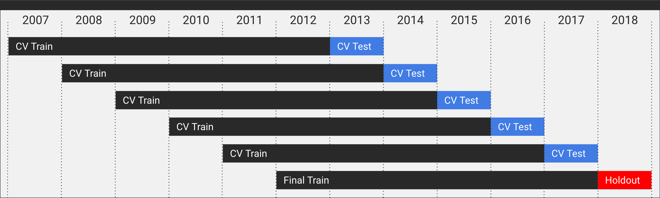
With a design matrix in place, it was time to split my data into a handful of training and testing sets for cross-validation along with a holdout dataset for final testing. Since this is a time-series prediction, I needed to ensure that there would be no data leakage from my testing sets into my training sets, so chose to break down the data into a series of rolling windows with 6-year long training sets and always predicting on the following year—in a production setting you would likely retrain significantly more often, but for this prototype that method was time and compute-prohibitive.

Modeling

It was nearly time to start training models—but which models to train? Rather than make that decision upfront, I built my modeling pipeline to flexibly accept a variety of classification models and parameters from sklearn's toolbox and planned to iteratively test these with my cross-validation sets and gradually eliminate models as I saw fit. Included in my testing were the following classifiers:

• Logistic regression
• K nearest neighbors
• Naive Bayes
• Support vector machine with linear kernel
• Support vector machine with radial basis function
• Random forest
• Gradient boosting
• Adaptive boosting
• Multi-layer perceptron with linear activation function
• Multi-layer perceptron with RELU activation function

Can I start teaching the robots now?

Data Processing

While my design matrix at this point was technically sufficient for modeling—that is, it was entirely numerical and had no null values—it still had a number of issues making it sub-optimal for modeling.

Inconsistent scaling

With features describing cancellation rates, precipitation, temperature, and more, the scales of my data were all over the place. To handle this, I used sklearn Standard Scaler module to rescale all of my features to be centered around a mean of 0 with a standard deviation of 1.

Too many features with not enough information

The model contained about 60 different features, many of them exhibiting high multicollinearity. Many of these were in fact constructions from the same data and similar-but-different interpretations of the same questions. To handle this, I applied two steps in series (though it took quite a bit of cross-validation for me to decided exactly how).

PCA

The first step I took was to apply principal component analysis to the data to reduce the dimensionality from 60 features down to 20 features. The theory behind this is that it should effectively collapse and combine my most similar features into new composite features that will capture the majority of the variance in the data in a more condensed form. While this technically results in a loss of resolution in the data, it also creates richer data more dense with information and proved to be more help than harm in my modeling.

It should be noted that while using PCA was helpful for condensing my features, a major downside to this action is that it severely reduces the interpretability of the model, as once the transformation has been applied it's no longer apparent which features are contributing most to a model's prediction.

Select K Best

The next step was to reduce that set of 20 features down to only those that conveyed the most information about whether or not a flight would be cancelled. To do this I utilized the SelectKBest module within sklearn and the f_classif function to compute the ANOVA F-value for each feature to determine the most predictive features to feed into the model. Ultimately after cross-validation I settled on using 12 features, but by no means did this seem to be a "clear winner".

Oversampling to restore balance

The dataset itself was highly imbalanced with respect to my target variable of cancellations. That is to say that since 99 out of every 100 flights isn't cancelled, a model could simply predict that a flight won't be cancelled every time and be 99% accurate while not actually doing anything useful. There are three ways to respond to an imbalanced dataset like this:

1. Do nothing.
2. Oversample the minority class until it's better represented.
3. Undersample the majority class to bring the two into parity.

As a lazy human, option 1 sure was tempting. But as an overachiever, I couldn't help but consider the others. I quickly observed that more data was better, so option 3 was out. That left option 2. I experimented with oversampling methods like SMOTE and ADASYN, but pretty quickly saw a fear of my come to fruition: by overrepresenting cancellations in my training set, I had trained my models to expect them far too often. This resulted in a very high number of false positives, which in this particular scenario is the worst case scenario. So I went back to step 1 and decided to do nothing about my imbalanced set.

Custom Score Function

Nearly ready to run my models, I found myself facing a critical question I'd been kicking around but putting off throughout the entire development process. How do I judge my models? While there are many standard responses out there for an imbalanced dataset (don't use accuracy, it's a trap!), how was I to know which one to use? I could use the F1 score, but giving equal weight to both precision and recall without a good reason feels awfully arbitrary. I could seek to maximize the area under the curve of my ROC score, but again, that's so divorced from the actual question I'm asking…so I did the natural thing and devised my own scoring metric.

I decided assign a cost/benefit value to each possible outcome of a prediction based on actual estimates of what these decisions would mean to an airline if they put the model into production. There are only four possible scenarios so…not too tough. Let me walk you through the reasoning.

• True Negative: The model correctly predicted that a flight that actually took off wouldn't be cancelled. An airline using the model wouldn't behave any differently in this circumstance, so this outcome incurs no effect on the score.
• False Negative (FN): The model incorrectly predicted that a flight that was actually cancelled would take off. An airline using the model wouldn't behave any differently in this circumstance, so even though the outcome is less than ideal, it incurs no effect on the score.
• False Positive: The model incorrectly predicted that a flight that actually took off would be cancelled. An airline using the model would mistakenly cancel the flight, incurring a heavy penalty cost, $\gamma_0$ which I'll elaborate on below.
• True Positive: The model correctly predicts that a flight that was actually cancelled would be cancelled. This is the holy grail, the real opportunity for savings. To quantify this, I made an assumption that with sufficient foreknowledge an airline could begin taking measures that would allow it to save some proportion of the expected losses due to cancellation, $\gamma_1$.

That might seem a bit long winded, but don't worry: it gets a bit worse before it gets better. I threw out those gammas to represent cost and benefit, but what are those really? I did a bit of research and number crunching to make some best guess estimates, and in a nutshell it looks a little like this. Based on data from this site:

• On average, a cancellation costs an airline about $5,770
• That can be narrowed down to about $3,205 for flights canceled due to an uncontrollable event like weather and more like \$9,615 if the cancellation was due to something the airline should have been able to control, such as missing flight crew or maintenance.
• What that means is that about 45% of costs incurred due to cancellations were avoidable
• This is extra money that goes towards things like inefficient usage of flight and maintenance crews as well as rebooking/reimbursing disgruntled passengers
• This means that on average about $2600 of the money lost due to a cancelled flight is money that the airline didn't have to lose. That's our margin to save from.

On a similar note, taking some averages from a variety of resources, we can estimate that an average flight has about 100 passengers on board and makes about $18 of profit per passenger. In other words, the average profit per flight is about \$1800.

Finally, there's that dangling $\gamma_1$ variable I threw out there. This is a wild assumption that would have to be manipulated in a production setting, and it's worth noting that all of my extrapolated interpretations hinge on this value. That said, I had to choose something. So what's it mean? I decided that a conservative estimate was that with sufficient foresight, an airline could maybe take back about 10% of that $2600 recoverable margin I mentioned above. In reality that might be 5 or 50, I'm not sure—but I went with 10.

With that in place, we can compute our cost of a false positive, which is the combination of lost profit plus the additional losses incurred by a cancelled flight (albeit a more efficiently cancelled flight, since we did it in advance). Skipping over the algebra, I can just tell you that it reduces to $\gamma_0 = \gamma_1 - \frac {profit} {margin} $.

To turn all of that into a usable score function, we add up the cost/benefit of every prediction in a test run and then finally normalize it against the total number of actual cancellations multiplied by our cost savings parameter, $\gamma_1$, like so:

$$ Score = \frac {\sum [\gamma_0 (FP) + \gamma_1 (TP)]} { \gamma_1 * (FN + TP)} $$

What this yields is a score where 0 means that the ultimate result would be that the airline sees no change in revenue, a negative number indicates that the airline would actually lose money by adopting the model, and a positive number (bounded at 1) represents the proportion of total possible savings the airline would be harnessing (i.e. a true positive rate of 1 would result in a score of 1).

Interpreting the Results

Okay, that was a mouthful, but also somewhat necessary. But now we can interpret our models! So how'd we do? It's quite tempting to describe the results as so-so, and that's not entirely wrong—but it's not entirely right either, so let's dig in.

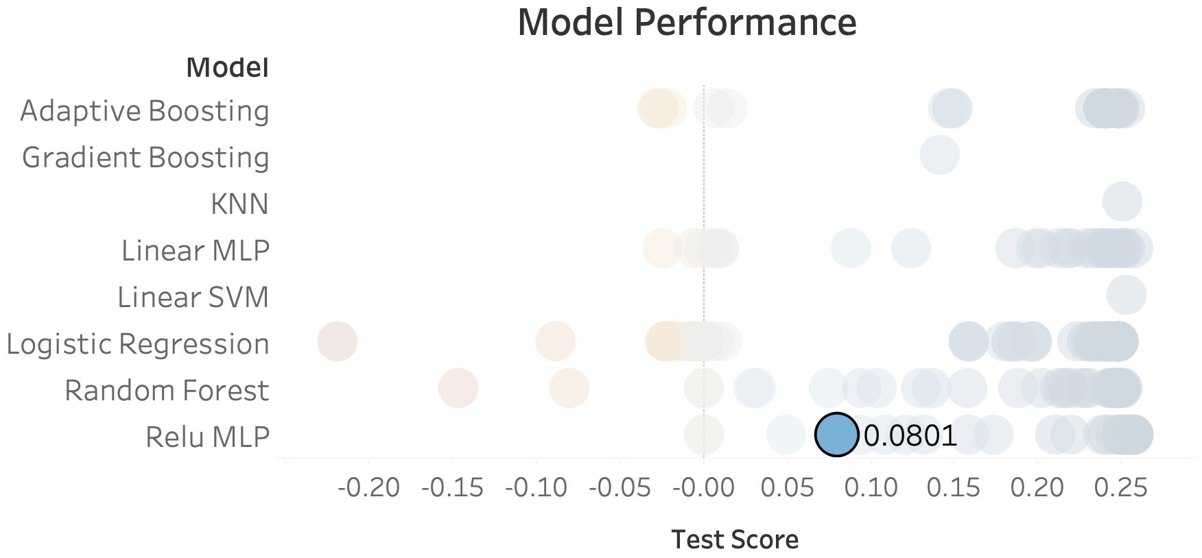
The chart above deserves a bit of interpretation. All the faded dots in the background represent average cross-validation test scores my models achieved with different parameters and inputs, and the highlighted result is the test score from the final run on my holdout dataset. Arguably, a jump from 0.25 down to 0.08 suggests that the model didn't generalize too well to 2018. And I don't thing that's wrong. So let's dive into a couple of these observations.

A point worth noticing is that pretty much all of the models seemed to plateau right around 0.25. Curious, eh? What that suggests to me is if there's a fundamental issue with the predictions it's not the models that are at fault but the features. It seems that the data on hand was able to predict about 25% of the reasons why flights would be canceled leading up to 2017, and that all of the models were able to identify those particular flights. However, it also seems that those other 75% of flights weren't being predicted at all, by any of the models, suggesting a lack of critical features. Furthermore, the fact that predictions on 2018 dropped so significantly suggest that something changed that the model couldn't keep up with.

Conclusion

The final result of a score 0.08 isn't stellar, but I think it's worth noting that it's not actually terrible either. Putting it into real world terms, this number means that my model correctly predicted 8% of all of SeaTac's flight cancellations in the year 2018 a full 24 hours before they happened. What's more, the model did this without making a single false positive prediction, which means that if airlines were utilizing the model, there would be zero mistaken cancellations and room for an estimated $12,000 in savings. Not an amount I'd get too excited about, but if you extrapolate that out to every airport in the US, now we're looking at more like a potential for around \$2 million dollars in savings per year. Not so shabby after all.

Future Work

This project was a fun prototype, but the conclusion certainly leaves a bit to be desired. That said, there's lots of room for improvement. Some obvious avenues to go down that I think would yield significant results include:

• Incorporating airplane-specific features, such as make/model and maintenance history
• Improved weather forecasting features
• Tailoring the cost function to take into account size of aircraft and number of passengers

Thanks for reading and feel free to reach out with questions or comments!